Excel VBA trick that helps you Convert an abbreviation into multiple words. From a merged cell to multiple cells!

This short Excel VBA project automates the task of converting abbreviations from a series of merged cells into their corresponding full words and then inserts those individual words into other cells.

Use: when it’s not as simple as
     A2 = B2,
     A3 = B3,
but more like:
    A2 = B2+B3+B4,
    A5 = B6+B7+B8,
and you’re dealing with text, not numerical values.
Functions and code used: VBA, multiple sheets, merged cells, arrays, for and if statements, CInt() and Mid$ functions.
Bonus: my trusty function to find last row or column in a sheet.
Audience: basic familiarity with VBA and/or some programming.

Background

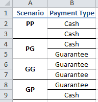
I had a sheet where I recorded results of payment test cases. Each Scenario entry represented a separate test case which could include multiple payment methods. The Scenario column had abbreviated payment types included in the particular case. Each record in Scenario column was a merged cell spanning over multiple rows to avoid repetition of the same data and easier visibility. P stood for Payment (Cash) and G stood for Guarantee. The table started pretty simple with only 4 scenarios.

My manager then decided that we needed to test as many as 6 different payment types for each test case. This meant a lot more test scenarios and a lot more complicated sheet. For 3 payments per case, there are 8 scenarios (PPP, PPG, PGG, GGG, GGP, GPP, GPG), for 4 payments, there are 16, and so on. It added up to 124 cases in total!

Number of payments per case	Number of needed scenarios
2	4
3	8
4	16
5	32
6	64

Now, the task of creating an Excel workbook to document each test case became a chore. This was going to be a very time consuming and error prone process.

If you’re wondering why the need for separate columns if they both contained the same data (one abbreviated, one not), each Scenario had additional information and was often repeated with different test specs. For example, Scenario 1: simple GP, Scenario 2: a GP where payee in P is different than the one used in G. Those details were kept in Scenario column as specs for each test case.

Since I was going to have multiple types of merged rows, I spread them into separate sheets – one sheet for 2 payments per scenario, one sheet for 3 payments, and so on. After I started to manually enter each possible Scenario, I dreaded having to do the same task in Payment type column. “There must be a better way to do this,” I thought and so I reached into VBA to automate this task.

There must be a better way to do this!

Overview of this Excel vba challenge

Here’s what we’ll need to automate the task of filling out Payment Type column:

1. Extract letters from Scenario column
2. Convert each letter into a full word (P into cash, G into Guarantee) and insert it into rows of Payment Type column
3. Repeat this process for all Scenarios and all sheets.

Our challenges:

#1 is pretty straightforward and can be achieved with an array although we want to limit contents of the array to only the abbreviation and ignore additional text after it.

For #2 we’ll need to know which row to insert a value into. Remember that Scenario column is merged. This process will not be a simple A2 = B2, A3 = B3,  but more like A2 = B2+B3+B4, A5 = B6+B7+B8, etc.

For #3 we’ll need to know where to start and where to end each iteration of #2. Scenario column is merged so on the sheet for 3 payment cases per scenario, Scenario cell will start on row 2, 5, 8, etc. We’ll also need to build in a way for our code to be flexible to the number of rows that are merged since that number will change from sheet to sheet.

---

Prep work:

Naming conventions: To simplify a process in later steps, I named the sheets in my workbook with the number corresponding to how many Payment Types per Scenario that sheet contains. My sheets are now named, 2, 3, 4, 5, 6.  If you must name your sheets differently, you’ll have to adjust some of the code accordingly.

Populate the columns of Scenario column before starting the next steps and be consistent. This means, no spaces before or between letters and start each cell with the abbreviations adding other text after.

Good: “PGP different payee for each”

Bad: ” PG P different payee for each”

Bad: “different payee for each PGP”

Start each module with Option Explicit. It’s a good practice and will help you from accidentally using undeclared variables.

---

1. Extract letters from Scenario column and place them in an array

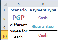
Example to visualize what we need to do: in a 3 payment type scenario, we will need to take the value of individual Scenario cell and populate Payment Type column.

To extract the value of Scenario cell, we need a simple .Value method. For start, we’ll keep it simple and start from a specific cell A2 (Cells(2, 1)). Variable targetRow is only temporary here. Later, we will put it in its own subroutine but for now, we’ll use it like this.

Dim targetRow As Long   ' move this later
targetRow = 2           ' move this later

Dim cellValue As String
cellValue = Cells(targetRow, 1).Value

I declared sheetName right in here also temporary. As we go further, we’ll take that line out of here and put it in another subroutine. Note: It has to be a string because Excel stores sheet names as strings, even if they’re numbers.

Dim sheetName As String  ' move this later
sheetName = "3"          ' move this later

We’ll hold the contents of Scenario cell as a string array so they can be used later for conversion.

Dim i As Long
Dim letterArray() As String
ReDim letterArray(CInt(sheetName) - 1)

CInt(sheetName) takes the string value of sheetName ("3") and converts it into an Integer (3). The size of the array is 2 (0,1,2) and hence -1 in our ReDim statement. This will stay the same no matter which sheet we will be working on (sheet "6" will have array size 5, etc).

Now, that declarations are out of the way, we can populate the array.

    For i = 1 To CInt(sheetName)
        letterArray(i - 1) = Mid$(cellValue, i, 1)
    Next

Mid$(cellValue, i, 1) function extracts the value of the Scenario cell (cellValue). This is how Mid$ function works (check out this source article for more info):

MID( text, start_num, num_chars )

text	The original text string.
start_num	An integer that specifies the position of the first character that you want to be returned.
num_chars	An integer that specifies the number of characters (beginning with start_num), to be returned from the supplied text.

Mid starts counting from 1 (not zero). So in our case, as it iterates through i starting from 1 to 3, it inserts individual letters into our array.

Note: this could be made easier but as you remember, my Scenario column sometimes contained more than just abbreviations and so I had to find a way to separate the Ps and Gs from the rest of the text.

---

2. Convert each letter in the array to a full word and insert it into rows of Payment Type column

The following is rather simple but took me a few tries to get right.

To convert, we’ll use a simple If statement. I had only two letters to cover so this was sufficient. If you have to work with more, a Case statement would work better.

To iterate through rows, I used a For statement but had to built in an additional If statement to stop the iteration

    For i = 0 To CInt(sheetName) - 1
         If letterArray(i) = "P" Then
              Cells(targetRow, 2).Value = "Cash"
         ElseIf letterArray(i) = "G" Then
              Cells(targetRow, 2).Value = "Guarantee"
         End If
         If i < CInt(sheetName) - 1 Then    ' prevent too many +1
               targetRow = targetRow + 1
         End If
    Next

Now, Cells(targetRow, 2) will point to the appropriate Payment Type row where we will paste the value we need. 

There were times, where I would have cells in my sheet which were blank and would cause the code to break. To omit those, we can check if cellValue is blank by wrapping creating an array and all for statements in an if statement:

If cellValue <> "" Then
     ' array and all of our for statements will go here
End If

Before proceeding to the next step, ensure that this code works for you. If not, place Breakpoints and step through your code in the debugger.

Option Explicit

Sub ConvertLetters()
' Below assumes that sheetName is an Integer stored as String
' sheetName should equal number of merged rows.

Dim targetRow As Long    ' move this later
targetRow = 2            ' move this later

Dim cellValue As String
cellValue = Cells(targetRow, 1).Value

Dim sheetName As String   ' move this later
sheetName = "3"           ' move this later

ActiveWorkbook.Sheets(sheetName).Activate

' if there's no value in column B, skip all
If cellValue <> "" Then
    Dim i As Long
    Dim letterArray() As String
    ReDim letterArray(CInt(sheetName) - 1)

    ' put letters into array
    For i = 1 To CInt(sheetName)
        letterArray(i - 1) = Mid$(cellValue, i, 1)
    Next

    ' translate array contents into corresponding Method (column 8)
    For i = 0 To CInt(sheetName) - 1
            If letterArray(i) = "P" Then
                Cells(targetRow, 2).Value = "Cash"
            ElseIf letterArray(i) = "G" Then
                Cells(targetRow, 2).Value = "Guarantee"
            End If
        If i < CInt(sheetName) - 1 Then ' prevent too many +1
            targetRow = targetRow + 1
        End If
    Next
End If
End Sub

3. Repeat this process for multiple rows

Now, that we have a working code that converts letters into words and puts them into correct cells, we need to iterate through the merged cells in Scenario column and repeat this process. Thankfully, this part is even easier. For this task, we’ll create a subroutine ConvertAll().

First of all, we’re going to need to find the last row for us to work with. There are different ways of finding the last row in a sheet but this particular function is what works best for me. Since I reuse it often, I keep it separate in a Functions module for easy access but you can keep it in the same module if you’d like. Send it a sheet name within your workbook and r and it will return the number of used rows in the sheet (in a Long format). It can also be used to find the last column – just send it a c.

Function LastRowColumn(sht As Worksheet, RowColumn As String) As Long

' Function that can return either the last row or column number through a user defined function for a given worksheet.
' INPUT: Worksheet name and "r" or "c" (to determine which direction to search)
' Example:
' lastRow = LastRowColumn(sheets("MySheet", "r"))

Dim rc As Long

' Taking only one character in case if you put in 'row' or 'column' instead of 'r' or 'c'

Select Case LCase(Left(RowColumn, 1)) 
  Case "c"
    LastRowColumn = sht.Cells.Find("*", LookIn:=xlFormulas, SearchOrder:=xlByColumns, _
    SearchDirection:=xlPrevious).Column
  Case "r"
    LastRowColumn = sht.Cells.Find("*", LookIn:=xlFormulas, SearchOrder:=xlByRows, _
    SearchDirection:=xlPrevious).Row
  Case Else
    LastRowColumn = 1
End Select
End Function

Now that you have my trusty LastRowColumn function, we can use it to find the last row in any of the sheets we’re working on.

Dim targetSheet As String
targetSheet = "3"    ' CHANGE MANUALLY if need to work on a different sheet
lastRow = LastRowColumn(Sheets(targetSheet), "r")

One problem you’ll run into here – the merged cells. In Sheet “3”, we have 25 rows but my trusty function returns 22 as the last row. How come?

This is because of how Excel stores values in merged cells. If you notice, when you highlight a few rows in a sheet and look at the name box in your ribbon, Excel displays the location of the first selected row, not the last.

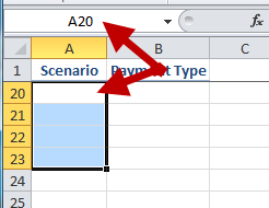
The same behavior applies to merged cells. The value of the merged cells is actually the value of the first merged cell.

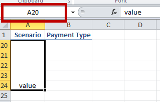
LastRowColumn() function searches for values in cells to determine last row. In our example, column A ends in a merged cell, and so it’s determined that the START of that merged cell is the end of the sheet. To fix this limitation, we simply need to add the number of merged rows. 

lastRow = LastRowColumn(Sheets(targetSheet), "r") + CInt(targetSheet)

Do you see now why I named my sheets as simple numbers? It keeps coming in handy.

Now that we have the correct last row, we’ll have to iterate through all Scenarios in the sheet with a For statement starting from Row 2 to lastRow. To do this, first we’ll make some changes to our ConvertLetters() subroutine. We want to be able to pass arguments to it like so:

For targetRow = 2 To lastRow
    Call ConvertLetters(targetSheet, targetRow)
Next

And so, we can remove targetSheet and targetRow declarations from ConvertLetters() moving them to our main subroutine ConvertAll(). 

---

The complete Excel VBA code:

Option Explicit
' Purpose of this module is to convert value of abbreviation contained within column Scenario into corresponding Payment Method.
' The number of merged rows has to be the same in a sheet.
' This should be done AFTER Scenarios are filled out (letters in column A) and BEFORE tests are performed.
' targetSheet's name MUST equal number of merged rows in the sheet.
' P = cash   G = Guarantee

Sub ConvertAll()
Dim targetRow As Long
Dim lastRow As Long
Dim targetSheet As String

' !!! ' targetSheet should be an Int stored as a string
targetSheet = "6" ' CHANGE MANUALLY if need to work on a different sheet

targetRow = 2       
lastRow = LastRowColumn(Sheets(targetSheet), "r") + CInt(targetSheet)  ' because of merging

For targetRow = 2 To lastRow
    Call ConvertLetters(targetSheet, targetRow)
Next
End Sub


Sub ConvertLetters(sheetName As String, targetRow As Long)
' Below assumes that sheetName is an Integer stored as String
' sheetName should equal number of merged rows.

Dim cellValue As String
cellValue = Cells(targetRow, 1).Value

ActiveWorkbook.Sheets(sheetName).Activate

' if there's no value in column B, skip all
If cellValue <> "" Then
    Dim i As Long
    Dim letterArray() As String
    ReDim letterArray(CInt(sheetName) - 1)

    ' put letters into array
    For i = 1 To CInt(sheetName)
        letterArray(i - 1) = Mid$(cellValue, i, 1)
    Next

    ' translate array contents into corresponding Method (column 8)
    For i = 0 To CInt(sheetName) - 1
            If letterArray(i) = "P" Then
                Cells(targetRow, 2).Value = "Cash"
            ElseIf letterArray(i) = "G" Then
                Cells(targetRow, 2).Value = "Guarantee"
            End If
        If i < CInt(sheetName) - 1 Then ' prevent too many +1
            targetRow = targetRow + 1
        End If
    Next
End If
End Sub

And that’s it. Isn’t it funny how attempting to explain this challenge took 10  paragraphs but the final code is only 42 lines long?

---

Did you find this article useful? Let me know in the comments.